| Species | Temperature Range | Depth Range |
|---|---|---|
| Oysters | 11-30°C | 0-70 m |
| Blue Mussel | 5-20°C | 0-60 m |
Have you ever considered the environmental impact of the food you eat? If you’re anything like me, you may have tried going vegan or vegetarian at some point, hoping to reduce your carbon footprint by cutting out beef and other protein sources often linked to greenhouse gas emissions. While individual choices are important, solutions that are practical and scalable—like marine aquaculture—can have a far more direct and meaningful impact on mitigating climate change.
What is marine aquaculture?
“Marine aquaculture refers to the breeding, rearing, and harvesting of aquatic plants and animals. It can take place in the ocean, or on land in tanks and ponds.” (NOAA Fisheries (2025)).
To many, farming in the ocean might sound novel, but it’s actually been a part of life in some regions for thousands of years. The Kwakwaka’wakw, the Indigenous people of the Pacific Northwest Coast, living in northern Vancouver Island and mainland British Columbia, were known for harvesting clams in clam gardens, sustaining their populations for thousands of years (Groesbeck et al. (2014)).
As the demand for seafood increases, reliance solely on wild-caught populations, which has been in steady decline since the 1980s (Aquarium of the Pacific (n.d.)) is not sustainable. Marine aquaculture has become popular for its use as a more suitable protein option than land-based meat production and wild-caught sources, with some studies showing that marine aquaculture greenhouse gas emissions could be 40% lower than emissions from land-based aquaculture (Arévalo-Martínez (2024)). It compliments current wild fisheries, produces jobs, and can meet the demand for seafood as human populations continue to grow.
As mentioned by Gentry et.al, limitations to marine aquaculture include ocean depth, marine protected areas, global fishing and shipping lanes, and environmental factors (Gentry et al. (2017)). The article mentioned that proper planning is key to successful marine aquaculture. That includes choosing the correct species based on environmental factors and the species’ suitability.
Overview of analysis
In this analysis, I investigated where to prioritize marine aquaculture in the West Coast of the United States within Exclusive Economic Zones (EEZ) for two focal species: oysters and blue mussels. Exclusive Economic Zones are regions of the ocean that are open for a country to explore and utilize for economic purposes. The U.S. West coast has five regions. (NOAA Ocean Service (2024)). Through the process of creating a generalizable function, I am able to visualize what suitable habitat is in reach for the country for marine aquaculture for any marine species.
The Data I Used
The data for this analysis includes a shapefile for the West Coast EEZ, bathymetry (depth) raster, and sea surface temperature raster.
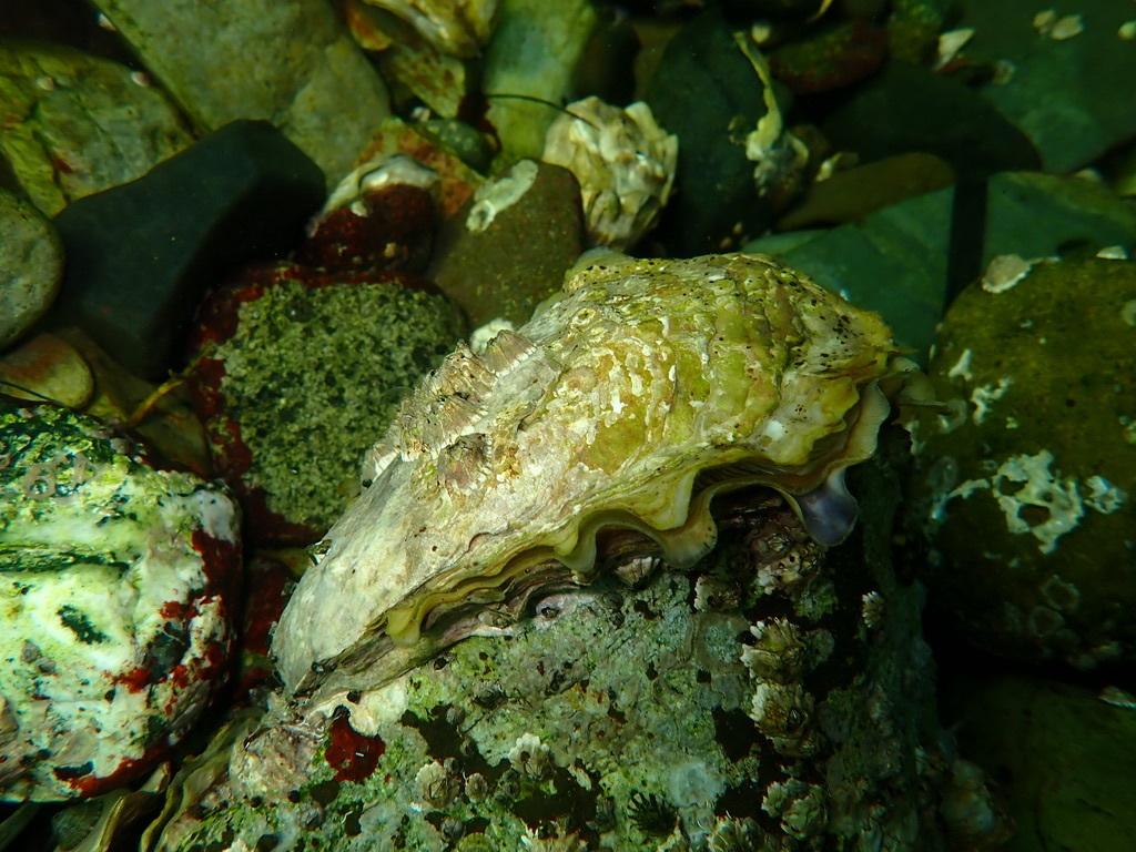
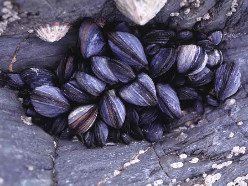
Focal Species
The two focal species for this study are oysters and blue mussels (Mytilus edulis). Both of these bivalve species are found in the Pacific ocean and have the ability to serve as a great protein source for marine aquaculture. I found their depth and temperature requirements from SeaLifeBase (n.d.) and Zagata et al. (2008).
Sea Surface Temperature Data
I will use average annual sea surface temperature (SST) from 2008 to 2012. The data is from NOAA’s Daily Global Satellite Sea Surface Temperature anomaly NOAA Coral Reef Watch (n.d.). I import this raster data as a raster stack with the rast() function from terra. While importing the data, I project the Coordinate Reference System (CRS) as EPSG:4326. This is the standard CRS for mapping.
Code
#......Import Sea Surface Temperature Data......

# Read in SST rasters in a raster stack
sst_fp <- list.files(here("posts", "marine-aquaculture-blog", "data"), pattern = "average_annual_sst_", full.names = TRUE)
# Stack
sst <- rast(sst_fp) %>%
  project("EPSG:4326") # project CRS

# Clear working environment
rm(list = 'sst_fp')
As with much environmental data, the SST data needs to be wrangled before I can utilize it. Firstly, the SST needs to be averaged for the years 2008 to 2012 and then converted from Kelvin to Celsius. This step is helpful by creating a single SST measurement that can be compared with the temperature requirements for my focal species.
#......Data Wrangling......

# Find the average sea surface temperature from 2008-2012
avg_sst <- mean(sst)

# Convert average SST from Kelvin to Celsius
avg_sst_c <- avg_sst - 273.15

# Clear working environment
rm(avg_sst)
Depth Data
I will use bathymetry (depth) data from the General Bathymetric Chart of the Oceans GEBCO Compilation Group (2022). This data also needs to be projected to the corrected CRS.
Code
#......Import Depth Data......
depth <- rast(here("posts", "marine-aquaculture-blog", "data", "depth.tif")) %>%
  project("EPSG:4326") # project CRS
In order to use the depth data with the sea surface temperature data, the resolution (number and size of pixels) and extent needs to match.
#......Crop depth raster......

# Create extent of 'avg_sst_c'
ext_sst <- ext(avg_sst_c)

# Crop depth raster to match the extent of the SST raster
depth_cropped <- crop(depth, ext_sst)

# Ensure data was cropped
if(ncell(depth) == ncell(depth_cropped)) {
  warning("data did not crop!")
} else {
  message("data cropped!")
}
data cropped!#......Resample......
# Resample to match resolutions
depth <- resample(depth_cropped, avg_sst_c, method = "bilinear") # method bilinear
# Check that the resolutions match
if (all(res(depth) == res(avg_sst_c))) {
message("Resolutions match!")
} else {
warning("Resolutions do not match")
}Resolutions match!# Remove 'depth_cropped' from environment
rm(list = 'depth_cropped')In order to work with this data spatially, the Coordinate Reference Systems need to match.
#......CRS check......

# Check that CRSs match
if (crs(depth) != crs(avg_sst_c)) {
  warning("Coordinate refrence systems DO NOT match!")
} else {
  message("Coordinate refrence systems match!")
}
Coordinate refrence systems match!Find suitable locations for species
With the sea surface temperature and depth data wrangled and ready to go, I will now find the suitable locations (area in km) that satisfy the specific sea surface temperature and depth range for oysters.
Reclassificaiton Matrix
In order to find suitable locations for the oyster, I need to reclassify avg_sst_c and depth data into locations that are suitable for oysters based on the specific requirements described in Table 1. Species Information. This is done with a reclassification matrix. This process simplifies the values within an object, it produces zeros and ones in the raster that satisfy specific criteria.
- 1: suitable locations
- 0: unsuitable locations
#......Reclassification matrix: sea surface temperature......

sst_matrix <- matrix(c(-Inf, 11, 0, # values -Inf to 11 = 0
                11, 30, 1,  # values 11 to 30 = 1
                30, Inf, 0), # values 30 to Inf = 0
              ncol = 3, byrow = TRUE)

# Apply the matrix to reclassify the raster, making all cells 0 or 1
sst_rcl <- terra::classify(avg_sst_c, rcl = sst_matrix)


# Assign Nan values as NA
values(sst_rcl)[is.nan(values(sst_rcl))] <- NA


# Ensure SST was reclassified
if (identical(values(avg_sst_c), values(sst_rcl))) {
  warning("SST not reclassified!")
} else {
  message("SST reclassified!")
}
SST reclassified!#......Reclassification matrix: Depth......
depth_matrix <- matrix(c(-Inf, -70, 0, # values -Inf to 70 = 0
-70, 0, 1, # values 70 to 0 = 1
0, Inf, 0), # values
ncol = 3, byrow = TRUE)
# Apply the matrix to reclassify the raster, making all cells 0 or 1
depth_rcl <- terra::classify(depth, rcl = depth_matrix)
# Ensure depth was reclassified
if (identical(values(depth), values(depth_rcl))) {
warning("Depth not reclassified!")
} else {
message("Depth reclassified!")
}Depth reclassified!I now have suitable locations for the sea surface temperature and depth specifications for oysters. I will do some further wrangling in order to be able to use this data for mapping. This includes multiplying the reclassification matrices (sst_rcl and depth_rcl) so suitable cells within each raster (‘1’ values) are kept and unsuitable cells (‘0’ values) are filled with NA values. I then find the area of suitable locations by using the expanse() function from terra and specifying the units to be in kilometers.
#......Find suitable locations......

# Multiply reclassification matrices to find suitable locations
# Creates matrix of 0/1 where 0 = not suitable and 1 = suitable
suitable_locations <- sst_rcl * depth_rcl


# Convert all zeros to NA values
suitable_locations[suitable_locations == 0] <- NA


# Find the area of suitable locations for oysters
suitable_area <- expanse(suitable_locations, unit = "km")
Determine the most suitable EEZ
I will determine the total suitable area within each EEZ for oysters. This data is from Marineregions.org Flanders Marine Institute (2025). EEZ vector data is read in as an sf object. Before I use this dataframe with my suitable_locations raster object, I need to ensure the CRS is defined as the same CRS I projected my depth and SST data to (EPSG:4326).
Code
#......Import Data and Check CRS......

# Import data
eez <- st_read(here("posts", "marine-aquaculture-blog", "data", "wc_regions_clean.shp"))

# Check if CRS match
if (st_crs(eez) == st_crs(4326)) {
  message("CRS match with depth and average sea surface temperature")
} else {
  warning("CRS does not match! Transforming required.")
}
I will now use my suitable_locations data frame to find the suitable locations within each EEZ. This is accomplished by using the terra function mask() which produces a new raster object with values in suitable_locations that intersect with eez.
#......Apply mask ......

# Mask suitable locations to eez habitat
eez_cells <- mask(suitable_locations, eez)

if (ncell(suitable_locations) == ncell(eez_cells)) {
  message("Mask worked!")
}else {
  warning("Mask did not work")
}
Mask worked!Now that I have the suitable regions within each EEZ (eez_cells). This is acompolished by calculating the area of each cell in eez_cells and rasterizing the eez object in order to use the zonal() function. zonal() is a function used to compute statistics with rasters. In this analysis, the function was used to keep cell areas only where EEZ cells are valid and sum them by EEZ.
#......Calculate total area ......

# make sure eez and eez cells extent match
if (ext(eez) == ext(eez_cells)) {
  message("Extents match!")
} else {
  warning("Extents don't match! Cropping eez_cells to match eez extent...")
  eez_cells <- crop(eez_cells, ext(eez))
}
Warning: Extents don't match! Cropping eez_cells to match eez extent...# Calculate cell size area of each raster cell
eez_cells_area <- cellSize(eez_cells, unit = "km")
#......Find total area......
# Rasterize eez
rast_eez <- rasterize(eez, eez_cells, field = "rgn_id")
# perform zonal operation
area_by_eez<- zonal(x = eez_cells_area * eez_cells, z = rast_eez, fun = "sum", na.rm = TRUE)Code
#......Join data......

eez_suitable_locations <- area_by_eez %>%
  left_join(eez, by = "rgn_id")

# clean up data frame

eez_suitable_locations <- eez_suitable_locations %>%
  rename(area_suitable_km = area) %>% # rename area
  select(rgn, area_suitable_km, geometry) # select for region, area, and geometry to plot

#.....Convert to sf object....
eez_suitable_locations <- st_as_sf(eez_suitable_locations)| Regions | Suitable Habitat (km) |
|---|---|
| Oregon | 1028.886 |
| Northern California | 194.126 |
| Central California | 3655.923 |
| Southern California | 3098.006 |
| Washington | 2421.627 |
Map: Oyster Suitable Area
In order to visualize the suitable habitat for oysters by each EEZ, I will produce a map. Maps like the following are helpful because they can break down information, such as the information in Table 2.Suitable Area for Oysters, in a way that is easy to interpret.
Code
oyster_map <-
  tm_basemap("Esri.WorldImagery") +
tm_shape(eez_suitable_locations) +
  tm_polygons(fill = "area_suitable_km" , # fill polygons based on suitable area
              style = "cont", # continuous value scale
    palette = c("#9ef7f0", "#1d524d"), # palette of colors
    title = "Suitable habitat (km²)", size = 0.8) + # legend title
  tm_layout(legend.outside = TRUE,
            legend.text.size = 0.5) +
  tm_title(paste("Suitable Habitat Range For", "Oyster Aquaculture", sep = "\n"), size = 1)  +
  tm_graticules(lwd = 0.2) + # gridlines
  tm_scalebar(position = c("left", "bottom"), text.size = 0.3)+ #scalebar
  tm_text("rgn", # overlay text for region
          size = 0.4,
          xmod = -0.2,
  ymod = 0.3)

# View map
oyster_map 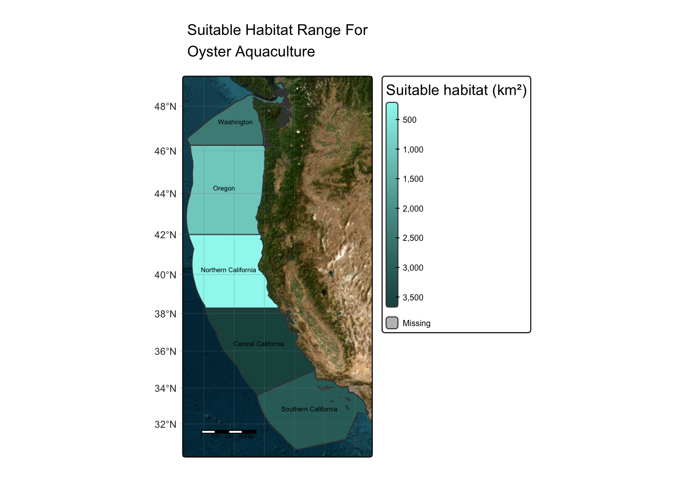
The map above depicts the suitable locations for oyster aquaculture within West Coast EEZs. As you can see, the regions with the most suitable habitat are Central and Southern California.
Generalizable function
Now that I have a worfklow for determining the suitable locations for oysters, I will create a generalizable function that can be applied to any species of interest. I will test this function for my second focal species blue mussels.
Code
# Define function name and arguments
suitability_fun <- function(sst_min, sst_max, depth_min, depth_max, species) {

# 1. Reclassification matrices

  # Define SST reclassification matrix
  sst_matrix <- matrix(
    c(
      -Inf,  sst_min, 0,   # below min sst = 0/unsuitable
       sst_min, sst_max, 1, # range of sst = 1/suitable
       sst_max, Inf,    0   # above max sst = 0/unsuitable
    ),
    ncol = 3, byrow = TRUE
  )

  # Define Depth reclassification matrix
dmin <- min(depth_min, depth_max) # ensure depth min is the smaller depth
dmax <- max(depth_min, depth_max)

depth_matrix <- matrix(
  c(-Inf, -dmax, 0,
    -dmax, -dmin, 1,
    -dmin, Inf, 0),
  ncol = 3, byrow = TRUE
)

# 2. Reclassify SST and Depth data

  # Reclassify SST
  sst_rcl <- terra::classify(avg_sst_c, rcl = sst_matrix)
  # Fill NAN values with NAs
  values(sst_rcl)[is.nan(values(sst_rcl))] <- NA

  # Reclassify depth
  depth_rcl <- terra::classify(depth, rcl = depth_matrix)

# 3. Find suitable locations
  # Multiply reclassifications to create matrix of 0/1
  suitable_locations <- sst_rcl * depth_rcl

  # Convert zeros to NAs
  suitable_locations[suitable_locations == 0] <- NA

  # Apply mask to keep only suitable raster cells in eez
  eez_cells <- mask(suitable_locations, eez)

  # Find cell area
  eez_cells_area <- cellSize(eez_cells, unit = "km")

# 4. Zonal operation

  # Rasterize eez
rast_eez <- rasterize(eez, eez_cells, field = "rgn_id")

  # perform zonal operation
area_by_eez<- zonal(x = eez_cells_area * eez_cells, z = rast_eez, fun = "sum", na.rm = TRUE)

# 5. Join data

eez_suitable_locations <- area_by_eez %>%
  left_join(eez, by = "rgn_id") %>% # join on 'rgn_id'
  rename(area_suitable_km = area) %>% # rename column
  select(rgn, area_suitable_km, geometry) # select certain columns for df

# 6. Convert to sf object
eez_suitable_locations <- st_as_sf(eez_suitable_locations)


# 7.  Create map

species_map <-
tm_basemap("Esri.WorldImagery") +
tm_shape(eez_suitable_locations) +
  tm_polygons(fill = "area_suitable_km" , # fill polygons based on suitable area
              style = "cont", # continuous value scale
    palette = c("#9ef7f0", "#1d524d"), # palette of colors
    title = "Suitable habitat (km²)", size = 0.8) + # legend title
  tm_layout(legend.outside = TRUE,
            legend.text.size = 0.5) +
  tm_title(paste("Suitable Habitat Range For", "\n", "Blue Mussel Marine Aquaculture"), size = 1) +
  tm_graticules(lwd = 0.2) + # gridlines
  tm_scalebar(position = c("left", "bottom"), text.size = 0.3)+ #scalebar
  tm_text("rgn", # overlay text for region
          size = 0.4,
          xmod = -0.2,
  ymod = 0.3)


# return species map and table of eez suitable area
return(species_map)

}
Apply function: Blue Mussels
I will now apply the suitability_fun function to my second focal species blue mussels to view blue mussel’s suitable habitat within West Coast EEZs.
suitability_fun(
  sst_min = 5, # define min stt value
  sst_max = 20, # define max sst value
  depth_min = 0, # define min depth value
  depth_max = 60, # define max depth value
  species = "Blue Mussel" # define species name
)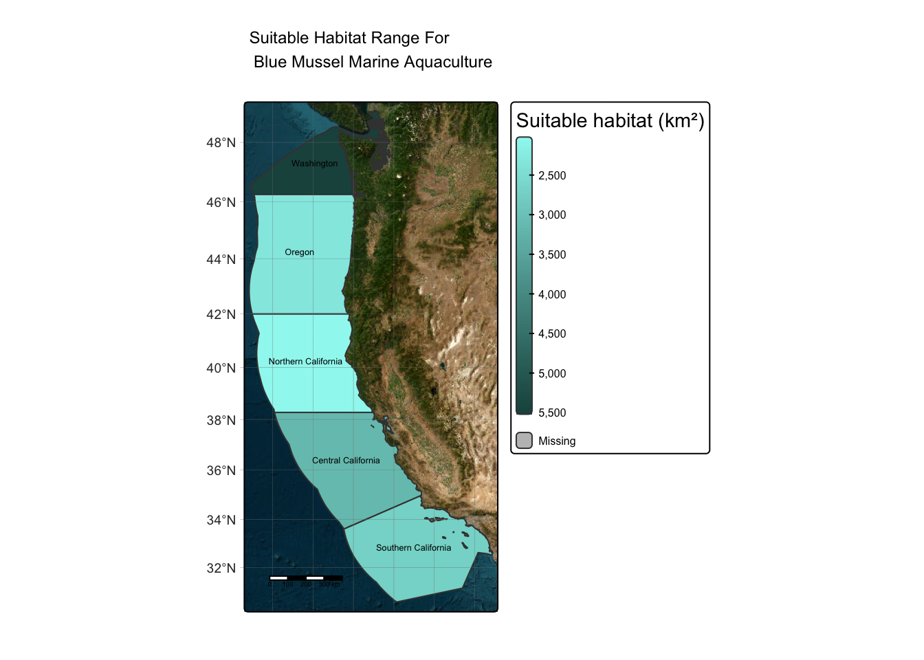
Reflection: The map above depicts the suitable locations for blue mussel aquaculture within West Coast EEZs. As you can see, the regions with the most suitable habitat are Washington. The rest of the California and Oregon coast contain less suitable locations probably due to the temperature range for blue mussels, whom prefer colder temperatures.
Final Thoughts
This project investigated the suitable habitats for two focal species –oyster and blue mussel– for marine aquaculture in West Coast Economic Exclusive Zones. Although I only mapped two species, the function suitability_fun can be used on a variety of species of interest for marine aquaculture. This analysis provides insight into the work needed to plan for marine aquaculture sites. Although I only include sea surface temperature and depth as specifications for suitability, as mentioned in Gentry et.al, there are many more factors that are of importance for assessing suitability of species. Additionally, as sea surface temperatures continue to rise due to climate change, the suitability for these species may alter.
References
Aquarium of the Pacific. n.d. “Marine Aquaculture.” n.d. https://www.aquariumofpacific.org/seafoodfuture/marine_aquaculture.
Arévalo-Martínez, D. L. 2024. “Offshore Aquaculture Greenhouse Gas Emissions Based on Ocean Net Primary Productivity.” Nature Food 5: 548–49. https://doi.org/10.1038/s43016-024-01005-x.
Flanders Marine Institute. 2025. “Maritime Boundaries Geodatabase: Exclusive Economic Zones (EEZ).” Data set. https://www.marineregions.org/eez.php.
GEBCO Compilation Group. 2022. “GEBCO_2022 Grid.” Data set. https://doi.org/10.5285/e0f0bb80-ab44-2739-e053-6c86abc0289c.
Gentry, Ryan R., Heike E. Froehlich, Danielle Grimm, Peter Kareiva, Michael Parke, Michael Rust, Steven D. Gaines, and Benjamin S. Halpern. 2017. “Mapping the Global Potential for Marine Aquaculture.” Nature Ecology & Evolution 1: 1317–24. https://doi.org/10.1038/s41559-017-0257-9.
Groesbeck, Amy S., Katherine Rowell, Dana Lepofsky, and Amanda K. Salomon. 2014. “Ancient Clam Gardens Increased Shellfish Production: Adaptive Strategies from the Past Can Inform Food Security Today.” PloS One 9 (3): e91235. https://doi.org/10.1371/journal.pone.0091235.
NOAA Coral Reef Watch. n.d. “5-Km Sea Surface Temperature Anomaly (SSTA) Product.” Data set. https://coralreefwatch.noaa.gov/product/5km/index_5km_ssta.php.
NOAA Fisheries. 2025. “Marine Aquaculture.” 2025. https://www.fisheries.noaa.gov/insight/marine-aquaculture.
NOAA Ocean Service. 2024. “What Is the EEZ?” 2024. https://oceanservice.noaa.gov/facts/eez.html.
SeaLifeBase. n.d. “Summary for Species #47622.” n.d. https://www.sealifebase.ca/summary/47622.
Zagata, C., C. Young, J. Sountis, and M. Kuehl. 2008. “Mytilus Edulis.” 2008. https://animaldiversity.org/accounts/Mytilus_edulis/.
Citation
BibTeX citation:
@online{segarra2025,
  author = {Segarra, Isabella},
  title = {Assessing {Potential} {Species} for {Marine} {Aquaculture} in
    {West} {Coast} {EEZs}},
  date = {2025-12-12},
  url = {https://isabellasegarra.github.io/posts/marine-aqaculture-blog},
  langid = {en}
}
For attribution, please cite this work as:
Segarra, Isabella. 2025. “Assessing Potential Species for Marine
Aquaculture in West Coast EEZs.” December 12, 2025. https://isabellasegarra.github.io/posts/marine-aqaculture-blog.